What is a Barnes-Hut Oct-Tree?

Barnes-Hut is a commonly used tree algorithm that represents a vast improvement over direct summation methods in the context of N-body computation. It is a hierarchical O(N log N) force-calculation algorithm invented by Josh Barnes and Piet Hut in 1986 (Nature, 324, 446). The algorithm reduces the number of computations by approximating far-field particles by their center of mass. To achieve this, the technique draws a hierarchical subdivision of space into cubic cells, each of which is recursively split into eight subcells (hence the name “oct-tree”) whenever more than one particle is found in the same cell.
Tree construction
The diagram below illustrates what a Barnes-Hut two-dimensional quad-tree would look like.

We have a sample distribution of 23 particles in a square box. The full domain is represented as the root of the tree on the right-hand side. Then we divide the domain evenly in four quadrants, and count how many particles are contained in each region. This constitutes the first level of our tree. To further illustrate this process, let’s focus on the lower left-hand-side quadrant (highlighted in purple.) We count four particles, and according to the prescription devised by Barnes & Hut, this means we need to keep subdividing until there is at most one particle per cell. Four levels are required to reach that stage, as shown on the right.
We have now constructed one section of the Barnes-Hut Oct-tree. The same process can easily be applied to the other quadrants in order to complete the representation of the entire particle distribution. But how does this hierarchical structure help us to calculate the force on a given particle?
Walking the tree to calculate the force
Barnes & Hut tell us that having constructed this tree, the force on any particle p can be approximated using a simple recursive calculation. Start at the root of the tree. Let l be the size or length of the cell currently being processed C, and D the distance from C‘s center of mass to p. If l / D < θ, where θ is an adjustable accuracy parameter ≈ 1, then approximate the particles in C by their center of mass. Otherwise, resolve C into its subcells and repeat at the next level.
Let’s focus on the particle highlighted in red in the diagram below and apply this process to calculate how much force it feels from the rest of the particle distribution.
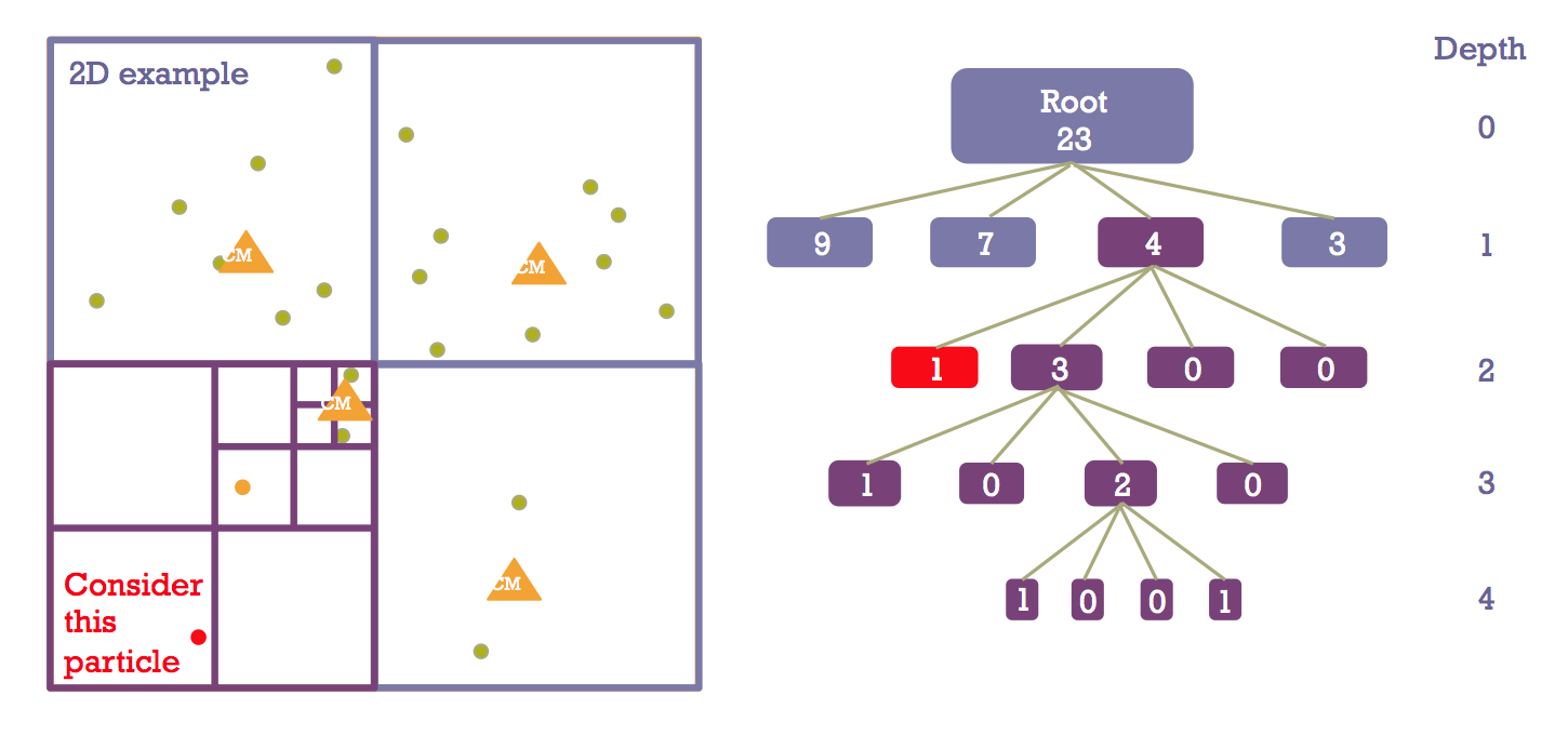
At level 1, the size of the 3 cells neighboring the one that contains p is smaller than the distance to p. As a result we approximate the force they exert by the center of mass. At level 2, two of the cells adjacent to the one that contains p are simply empty, so we leave them alone. The third one however contains 3 particles and its size to distance ratio is too large to be approximated. Moving on to the next level, the cell containing 2 particles is distant enough to be treated approximately, while the closer particle must be taken into account individually.
In this sample problem, we’ve reduced the number of force calculations from 22 for a direct summation scheme, to 5 using a quad-tree. The accuracy and computational load tradeoff can be tuned adjusting the parameter θ. Now let’s imagine we have many particles. We need to repeat the process of:
- Constructing the tree
- For each particle, walking through the tree to calculate the force
… at each timestep. This can be done serially (see our code repository for the serial version); still, it is a computationally intensive problem asking to be parallelized. If each process is in possession of the oct-tree, then step 2 is embarrassingly parallel. Parallelizing step 1 is less obvious. Let’s look at our approach to this problem with MPI.