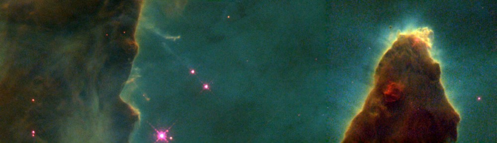
The Pillars of Creation is a false colour image with SII 6176/6731 Å in red, Hα 6536 Å in green, and OIII 5007 Å in blue. To determine the properties of the photoevaporative flow, Hester et al. used a spectral synthesis code (Cloudy 85) to predict the emission from these lines from different models of the nebula. The interactive nebula predictor shows the output of a grid of Cloudy 13 models.
An important part of predicting the spectrum is the radiative transfer equation, with the incoming radiation determined by the star:
$latex \frac{dI_{\nu}}{ds} = -I_{\nu} \frac{d\tau_{\nu}}{ds} + j_{\nu} &bg=0f0f0f&fg=ffffff&s=3 $
Photoionization absorbs radiation:
$latex \frac{d\tau_{\nu}}{ds} = \sum\limits_{X,i} n(X^{+i})a_{\nu}(X^{+i})&bg=0f0f0f&fg=ffffff&s=3 $
Recombination provides emissivity:
$latex j_{\nu}(X^{+i},T) = \frac{2h\nu^{3}}{c^{2}} (\frac{h^{2}}{2\pi mkT})^{3/2}a_{\nu}\exp(-\frac{h(\nu-\nu_{0})}{kT})n(X^{+i})n(e)&bg=0f0f0f&fg=ffffff&s=3 $
In practise, only hydrogen and helium need to be included in radiative transfer because of their overwhelming abundances.
To determine the abundances of the different ionization states of each species, ionization equilibrium is used. In any place in the nebula for each ionization state, ionizations (left hand side) are balanced by recombinations (right hand side):
$latex n(X^{+i})\int\limits_{\nu_{0}}^{\infty}\frac{4\pi J_{\nu}}{h\nu}a_{\nu}(X^{+i})d\nu = n(X^{+(i+1)})n(e)\alpha_{G}(X^{+i},T) &bg=0f0f0f&fg=ffffff&s=3 $
The temperature is determined by thermal equilibrium for the gas:
$latex G – L_{R} = L_{FF} + L_{C} &bg=0f0f0f&fg=ffffff&s=3 $
With G being energy input from photoionization, LR being energy losses from recombination, LFF being energy losses from free-free radiation, and LR being energy losses to collisionally excited lines. Each of these terms as a sum over all species and ionization states.
When a photoionization occurs, the excess energy h(ν–ν0) of the photon comprises the kinetic energy of the freed electron:
$latex G(X^{+i}) = n(X^{+i})\int\limits_{\nu_{0}}^{\infty}\frac{4\pi J_{\nu}}{h\nu} h(\nu-\nu_{0}) a_{\nu}(X^{+i})d\nu &bg=0f0f0f&fg=ffffff&s=3 $
When a recombination occurs, the kinetic energy of the electron 1/2 m v2 is lost from the gas:
$latex L_{R}(X^{+i})=n(X^{+(i+1)})n(e)\int\limits_{0}^{\infty} \sigma(X^{+i},v)v \frac{1}{2}mv^{2}f(v)dv &bg=0f0f0f&fg=ffffff&s=3 $
LR < G because slower electrons are preferentially captured.
Electrons and ions will scatter off each other, releasing some radiation:
$latex L_{FF}(X^{+i}) = \frac{32\pi e^{6} i^{2}}{3^{3/2}hmc^{3}} (\frac{2\pi k T}{m})^{1/2}g_{FF}n(e)n(X^{+(i+1)}) &bg=0f0f0f&fg=ffffff&s=3 $
In the above three mechanisms, only hydrogen and helium are important because of their abundances.
Metals, however, have many collisionally excited lines and thus contribute to LC. The atoms and ions in the gas can be excited or de-excited by radiation (A terms) and collisions (q terms). Transitions from excitation state j to k (left hand side) must be balanced by transitions from excitation state k back to j (right hand side), determining the population nj of each state of species X+i:
$latex \sum\limits_{k}n_{k}n(e)q_{kj} + \sum\limits_{k}n_{k}A_{kj} = \sum\limits_{k}n_{j}n(e)q_{jk} + \sum\limits_{k}n_{j}A_{jk} &bg=0f0f0f&fg=ffffff&s=3 $
Then, spontaneous de-excitations from each state determine the cooling rate:
$latex L_{C}(X^{+i}) = \sum\limits_{j}n_{j}\sum\limits_{k<j}A_{jk}h\nu_{jk} &bg=0f0f0f&fg=ffffff&s=3 $
These equations must be solved iteratively. To start, the “on-the-spot” approximation can be made, which assumes that photons coming from recombination are immediately absorbed. Thus, the radiation intensity at any point is the sum of intensity from the star (first term) and from local recombinations:
$latex J_{\nu} = \frac{\pi F_{\nu,\star} R^{2}}{r^{2}} \exp(-\tau_{\nu}) + \frac{j_{\nu}}{\sum\limits_{X,i} n(X^{+i}) a_{\nu} (X^{+i})} &bg=0f0f0f&fg=ffffff&s=3 $
Then the ionization and thermal equilibrium equations can be integrated outwards from the star to get approximate ionization populations n(X+i) and temperature T at each point in the nebula. Then the radiative transfer equation can be integrated using these approximate solutions, and then the ionization and thermal equilibrium conditions re-integrated using the new radiative transfer solution for Jν. This procedure can be iterated until the solution converges.
(For more details on modelling nebular structure, consult Osterbrock & Ferland’s Astrophysics of Gaseous Nebulae and Active Galactic Nuclei.)
Now take a closer look at “The Pillars of Creation” to see how these models of nebular structure help us understand the properties of the Eagle Nebula.